Opening the Black Box

Natural gas and electric utilities have always been concerned about reliability and safety, and each year spend billions of dollars repairing and replacing transmission and distribution assets. However, unlike the commodities they sell, there are no markets to value safety and reliability. Utilities can’t purchase these attributes directly, but instead must determine the best targets for each, while constrained by available resources. There are no guarantees. No system is 100 percent safe or reliable. No amount of planning or investment can completely eliminate sudden, unplanned equipment failures. 

In fact, reliability and safety share characteristics of public goods. Customers along a specific distribution line, for example, can’t choose different levels of reliability; it’s the same for all of them. Thus, utilities must somehow determine how best to provide needed safety and reliability at the lowest possible cost. And state utility regulators must be able to evaluate those determinations accurately and independently. 

Many utilities have developed their own methods to address the inevitability of equipment failure and evaluate the tradeoffs between replacing and repairing aging assets. Others rely on methods developed by consultants. Some of these methods are simply ad hoc – e.g., “replace utility poles that are 30 years old” or “test underground distribution lines every five years.” And these ad hoc rules can, in some cases, appear to work well. Yet they aren’t based on sound engineering and economic principles. Utilities that employ such rules can’t know whether they provide a least-cost strategy. Furthermore, such rules are less likely to pass the heightened regulatory scrutiny that comes when budgets are stretched. In other cases, utilities rely on flawed analytical tools. These tools, while not ad hoc, can lead to worse decisions, if flaws appear in underlying assumptions or analytical approaches. 

Although the comprehensiveness of these methods varies, they all lead to inefficient or, worse, incorrect, decisions. In other words, utilities can end up spending more money than needed to achieve desired levels of safety and reliability. Or, they obtain less reliability and safety than their methodologies claim to provide. In either case, both ratepayers and utility shareholders lose: with ratepayers paying more and investors seeing lower returns if certain investments are disallowed by regulators.

With natural gas and electric utilities spending billions each year on transmission and distribution systems, both for new equipment and repairs to the old, even small improvements in asset management strategies can yield significant savings for consumers, while maintaining or improving overall reliability and safety. Here we introduce an approach that avoids errors common to other asset management approaches. Our methodology combines advanced statistical and mathematical optimization techniques. It recognizes the interdependence between asset management strategies and testing regimes. It also recognizes interdependencies among assets themselves and avoids the errors common to other asset management approaches. 

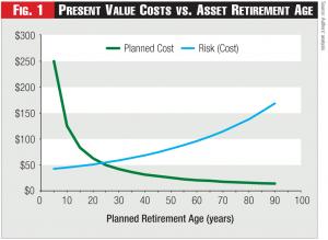Figure 1 - Present Value Costs vs. Asset Retirement Age

For utilities and their shareholders, our methodology can provide greater assurance that asset management decisions are prudent, so that the costs can be recovered from ratepayers, thus reducing uncertainty. For utility regulators, the methodology provides greater assurance that utilities are providing required levels of safety and reliability at the lowest cost, thus benefitting ratepayers. Moreover, the methodology can also provide regulators with an objective ability to independently verify utility asset management strategies, rather than accept black-box approaches they can’t assess independently.

First, we describe six common errors in models used to make asset management decisions for transmission and distribution (T&D), and how these errors lead to inferior decisions about equipment repair and replacement. Second, we explain the four uncertainties that increase the complexity of asset management strategies. Third, we describe the analytical method we developed that addresses these uncertainties in a statistically and mathematically correct way. We conclude with a real-world application of the methodology, showing how it’s been used by one regional transmission organization (RTO) to evaluate optimal numbers and locations of spare transformers. 

The Cost-Risk Tradeoff

Decisions regarding whether to repair or replace specific assets, or simply leave them in place, share common characteristics and tradeoffs. The basic tradeoff is well-known to anyone who owns a car: putting off replacement to postpone the cost of buying a new one must be tempered against the increasing cost of likely repairs. For utilities, which operate assets over the indefinite future, an asset management strategy based on extending the life of an asset reduces the present value of the cost of asset replacement over the indefinite and foreseeable future. However, as assets age, they tend to require more expensive and more frequent repairs. Further, taken to its logical conclusion, extending the life of an asset tends to provide a “run-to-failure” asset management strategy. Therefore, evaluation of life extension or run-to-failure strategies must address the cost of unplanned failures. These concepts are illustrated in Figure 1. 

Figure 1 illustrates the decreasing present value cost associated with planned asset replacements as a function of asset retirement age: the greater the age at which an asset is retired, the lower the present value cost of a timed sequence of asset replacements over the indefinite future. However, as an asset’s retirement age increases, the higher the risk (and unplanned costs) associated with repairs or asset failure that could occur in each increasingly large replacement cycle. The costs shown are only expected values, because when (or if) an asset fails is uncertain. The likelihood of an asset’s failure sometime in the future is called the asset’s “hazard rate.”¹

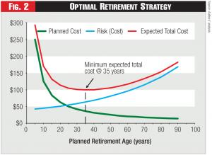Figure 2 - Optimal Retirement Strategy

The optimal retirement age is defined as the one for which the expected total cost is minimized. This is shown in Figure 2. The expected total cost is the sum of the planned replacement costs and the expected cost of asset failures (risk). In the example presented in Figure 2, the minimum expected cost occurs at a planned retirement age of 35 years for this type of asset.²

Defining and identifying the optimal replacement strategy is conceptually straightforward, as shown in Figure 2. However, it turns out that Figure 2 illustrates the flaws of commonly applied methods. The reason is that Figures 1 and 2 can’t be used in practice to find the optimal retirement age for an asset. In other words, one can’t simply construct the two curves and read off the optimal retirement age. Yet, this is commonly done, based on four incorrect assumptions: 1) the time interval between replacements is always the same; 2) all replacement life-cycles cost the same; 3) the actual timing of asset replacements within each replacement life cycle is always the same; and 4) the actual capital costs of asset replacement due to unplanned failures aren’t considered, leading to underestimates of actual capital costs. 

Some Common Mistakes

We have also identified at least six common types of errors present in many commonly applied asset management methodologies (sometimes also called “repair or replace”) that lead to inferior solutions. These common errors include: 1) ignoring or wrongly defining the initial conditions of assets being evaluated; 2) using a misleading concept of “asset health” to lump different classes of assets together; 3) applying a static method (i.e., one that doesn’t recognize how the condition of an asset changes over time), based on asset health, to determine how to treat an asset; 4) conflating asset condition with the consequences of asset failure; 5) failing to account for all of the costs of asset failure; and 6) failing to integrate testing policies into an overall asset management strategy. 

Any method that fails to assess the initial condition of assets, or assesses them incorrectly, can’t possibly identify an appropriate management strategy and, as a consequence, will be ad hoc.

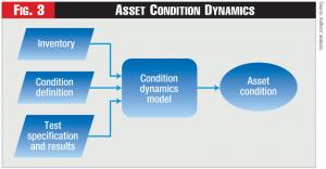Figure 3 - Asset Condition Dynamics

Consider, for example, wooden utility poles. Unless a pole has fallen over or is leaning precipitously, it’s difficult to determine its condition. A pole might look fine on the outside, but be rotten inside, awaiting the next windstorm or errant automobile to knock it over. A pole replacement strategy based on whether the pole looks “good” on the outside, regardless of its true internal condition, will lead to excessive pole failures, more outages, and higher costs.

And a wooden utility pole tested and found rotten is far more likely to fail at any given time. That is, asset condition determines the likelihood of future failure. This likelihood is known as a “condition-dependent hazard rate.” Although a common-sense way to characterize the so-called “health” of an asset is to measure its remaining life, this straightforward idea has been expanded to include many other aspects of an asset into a single measure called “asset health.” However, it turns out that the optimal repair-replace strategies for assets having the same health can be quite different. 

Typically, asset health measures combine several distinct attributes, such as age and near-term failure likelihood, into a single measure. However, such a single measure can be misleading because different assets with different attributes could have the same asset health. For example, an older, well-maintained transformer, for example, might have a much lower hazard rate than a younger, poorly-maintained one. Thus, these assets determined to have the same overall health might, in fact, need to be treated very differently. 

In some cases, the asset health measurement conflates both the likelihood of near-term failure and the consequences of failure. But that can lead to incorrect conclusions. Consider, for example, a car’s tires. Most of us would agree that replacing worn tires before they fail is a better strategy than waiting for a blowout, which can have severe consequences. However, keeping a worn spare tire can be a reasonable strategy because the consequences of tire failure can be managed as well with a worn spare as a brand new spare because both enable one to drive to the nearest tire store. Thus, the asset management policy associated with a tire’s condition depends on the tire’s intended use, not just the immediate failure rate and the consequences of failure. 

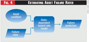Figure 4 - Estimating Asset Failure Rates

Yet another problem is that asset health measures typically fail to account for the dynamics of asset condition; i.e., how an asset’s condition changes over time. The condition of an asset changes not only naturally as it ages, but also because of how it’s operated and maintained. Again, a car engine is a good example: its condition depends not only on its age, but on how much it’s run, whether the car is driven in stop-and-go traffic or primarily on the highway, how frequently the oil is changed, and so forth. Therefore, the asset’s hazard rate will change over time as the asset’s condition changes. An asset management strategy that assumes the hazard rate doesn’t change over time won’t be least-cost.³

Nor should asset health standing alone dictate asset-management strategy. For example, in some cases, utilities will rank T&D assets by their health and replace those assets in order until the utility reaches a predetermined budget amount. Thus, asset health is treated as if it were a benefit-cost ratio. However, ranking alternatives based on benefit-cost ratios is itself generally inaccurate.⁴

Utilities also might fail to consider all failure costs. For example, widespread power outages can garner negative publicity and additional regulatory scrutiny of a utility’s actions. In other cases, such as with the gas pipeline explosion at San Bruno, California, regulators can levy multi-million dollar fines, as the California Public Utilities Commission levied against PG&E.

Finally, asset testing is also crucial to asset management. It’s impossible to determine a least-cost asset strategy without also determining the optimal asset testing regime. In other words, asset strategy and testing strategy are interdependent. We have found, for example, that utilities often test too frequently or rely on the wrong kinds of tests. An optimal asset management strategy must account for the outcomes of tests because those outcomes provide information about the true condition of the assets. That’s another reason for rejecting a static method of asset management, such as ranking assets by asset health, in favor of a dynamic one that reflects changing conditions over time. 

A Dynamic Alternative

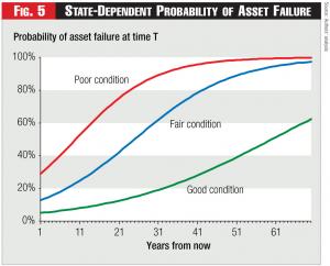Figure 5 - State-Dependent Probability of Asset Failure

These problems lead us to propose an alternative approach – which we call a dynamic optimization methodology to determine asset strategy.⁵  This type of dynamic strategy addresses four types of uncertainty: 1) uncertainty regarding an asset’s current condition and how that condition changes over time; 2) uncertainty regarding the accuracy of tests of an asset’s condition; 3) uncertainty regarding an asset’s remaining life; and 4) uncertainty regarding the effects of repairs on an asset’s condition and, therefore, its remaining life.⁶

As we discussed previously, determining an optimal asset management strategy requires that we determine how an asset’s condition changes over time, because the condition of an asset at any time t determines the probability of failure thereafter. To do this, we combine condition definitions (e.g., what does it mean for an asset to be in good condition today?) with tests that can evaluate the asset’s condition. These are combined to establish what we call a “condition dynamics model (CDM).” The CDM determines how an asset’s condition is likely to change over time, given its current condition.⁷ (See Figure 3).

However, knowing an asset’s condition today – unless it’s already failed – and the forecast of asset condition given by the CDM won’t provide enough information to make asset management (repair, replace, test, do nothing) decisions. That requires a model that estimates the likelihood of asset failure tomorrow, given an asset’s condition today. Such models are called State-Dependent Hazard Rate Models, as shown in Figure 4.

Figure 5 illustrates three hazard rates for a class of assets in different condition today.⁸ Although it’s straightforward to determine a repair-replacement strategy along a single hazard function, that strategy won’t be least-cost because we further recognize that repairing an asset can also change its condition and thus change the appropriate hazard rate. Depending on the type of repair made, however, there will also be uncertainty as to what is that new post-repair condition.⁹

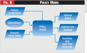Figure 6 - Policy Model

For example, suppose your car is running poorly and you ask the mechanic to change the car engine’s oil. Changing the oil will improve the engine’s condition because old oil has various contaminants that can increase wear on the various moving parts. However, if the engine has leaking rings or a blown gasket, changing the oil will do little to improve its condition. Thus, a simple repair can still leave a high level of uncertainty as to the engine’s true condition. If, on the other hand, you ask the mechanic to completely rebuild your car’s engine, the engine will be in good condition with no uncertainty (assuming the mechanic has rebuilt it correctly). The optimal engine repair strategy, therefore, depends on the type of repair made and the effect of that repair on the engine’s condition. Moreover, an optimal strategy must evaluate the tradeoffs between the cost of the repair made and the (uncertain) impact on the engine’s post-repair condition.¹⁰

Developing an optimal policy for each class of assets requires additional information, including: 1) the available types of repairs (e.g., major? minor?); 2) the type of replacement asset (e.g., the same asset type? an improved asset?); 3) the costs of the different alternatives; and 4) the probability distribution of the cost of failure. Moreover, the optimal policy includes determining the optimal testing policy, based on the accuracy and the cost of alternative testing regimes. Thus, the Policy Model, shown in Figure 6, can determine the optimal policy as well as the expected benefit of alternative testing regimes. The Policy Model also forecasts the behavior of the asset inventory and the cash flows associated with implementing the optimal policy. 

The Policy Model can be envisioned as a type of decision tree. For example, suppose we have a high-voltage transformer, which we believe is in fair condition today (Time =0). The transformer can be replaced, overhauled, or simply left alone (the “Do Nothing” alternative), as shown in Figure 7.

In the figure, after overhauling or doing nothing, there will remain uncertainty as to the transformer’s actual condition at Time = 1. Specifically, if the transformer is overhauled, its condition either will be good with probability PO (good) or fair with probability PO (fair).¹¹ However, if the transformer is left alone and doesn’t fail, next period it will be either in fair condition with probability PN (fair) or poor condition with probability PN (poor). The relative likelihoods of the resulting conditions in the Do-Nothing case are determined by the Condition Dynamics Model. The relative likelihoods associated with the overhauling procedure are based on utility-specific or industry-wide knowledge of the outcomes of overhauling

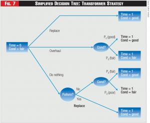Figure 7 - Simplified Decision Tree: Transformer Strategy

In actuality, of course, we are dealing with multiple uncertainties, including whether to test the transformer’s condition and, if so, what type of test to undertake. Moreover, the time horizon used by the model is infinite. The actual model uses dynamic optimization techniques to solve the model for each asset class and develop a recommended strategy, including a testing strategy. Moreover, the model can estimate the value of different testing regimes.

Spare Transformer Inventory Analysis 

One aspect of ensuring a reliable electric system is quick restoration from forced outages. This type of repair-replace decision involves the value of spare equipment, similar to the spare tire example discussed above, with an additional geographical component. 

For one RTO, a key issue was the best management policy for the step-down transformers on its system, which reduce voltages from 500 kV to 230 kV. Specifically, the RTO had four questions: 1) how often should these transformers be tested? 2) when should they be overhauled (refurbished)? 3) when should they be replaced? and 4) where should spare transformers be deployed to mitigate the consequences of transformer failures?

The expected value of a spare at a given location within the RTO is based on several factors. Not surprisingly, the first factor is the expected value of reduced outage duration. Thus, if the cost of a forced outage at location X is $OX per hour, then the expected value of the spare, E(VS,X), equals the probability of failure, PX(f), times the expected reduction in outage time because of locating the spare at X, ∆TX, times the outage value, i.e., E(VS,X) = Px (f)•∆TX•$0X. 

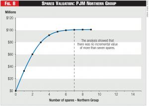Figure 8 - Spares Valuation: PJM Northern Group

In addition to this value, however, a spare will have additional incremental value in one area if it can mitigate the consequences of transformer failure elsewhere. This means one can’t simply add up the expected value of spares at each location to determine the overall expected value of locating spare transformers at every location. For example, if a transformer at location X fails, but transformers in nearby locations A, B, and C can handle the additional loads, then the value of a spare transformer at X will be reduced if there are already spares located at A, B, and C. 

For the RTO analysis, step-down transformers were grouped into geographic areas. For example, the “Northern Group” consisted of transformers at 18 separate substations. To mitigate failure risk, the RTO had located one spare transformer at each of the substations.

The value of locating a first spare at each location was then calculated. The analysis showed that locating a spare at “Lovell”¹² had a net expected value of $29.5 million,¹³ larger than the incremental values at any other location. Moreover, the analysis showed that, because siting a first spare at Lovell also provided additional risk mitigation benefits in the event of transformer failures at other locations, the overall expected net benefit of siting the first spare at Lovell was $32.8 million.

Next, the analysis determined the optimal location of siting a second spare, given that the first spare was already sited at Lovell. This analysis showed that siting a second spare at “Elgin” had an expected value of $27.4 million. The process continued, each time calculating the incremental expected value provided by the next spare, given the spares that had been sited. In total, the analysis showed that there was no incremental benefit to siting more than seven spares in the entire group, as shown in Figure 8. Moreover, the analysis determined that locating a second spare at Elgin had greater value than siting a first spare at many other locations in the Northern Group. Thus, rather than using 18 spares, one at each location, the analysis freed up 11 spares, which the RTO then relocated. In fact, approximately two weeks after the RTO relocated one of the redundant spares to a location in a different transformer group, as recommended by a subsequent analysis, the existing transformer at that substation failed. Because of the location recommendation, the RTO was able to restore service far more quickly and minimize the consequences of the transformer’s failure.

Endnotes:

1. The hazard rate, h(t), measures the probability that an asset will fail shortly after time t, given that it’s survived until time t. The hazard rate can be found empirically by estimating the survivor rate, S(t), which is the probability that an asset survives until at least time t. Mathematically, for some small interval Δt that begins at time t, the probability of failure during this small interval of time = h(t)Δt , where h(t) = [dS(t)/dt ]/S(t).

2. At the optimal retirement age, the expected present value marginal cost from higher risk equals the expected present value marginal benefit from fewer replacements; i.e., the slopes of the curves are equal in magnitude and opposite in sign. Note that the optimal replacement age generally isn’t where the planned cost and risk cost curves cross.

3. For those who are mathematically inclined, finding the least-cost strategy over time is known as an “optimal control problem.”

4. For a brief discussion, see Leonardo R. Giacchino and Jonathan A. Lesser, Principles of Utility Corporate Finance, chapter 17, Public Utilities Reports, Inc., 2011.

5. The Appendix to this article provides a formal mathematical description of the modeling structure.

6. For further discussion, see Charles D. Feinstein and Peter A. Morris, “The Role of Uncertainty in Managing Aging Assets In Electric Utility Systems,” IEEE PES Transmission and Distribution, New Orleans, April 2010. A copy of this presentation is available from the authors.

7. Technically, the CDM establishes a Markov-chain type of probability model, in which we estimate the probability of moving from state A to state B. For example, the probability of a transformer in good condition today being in fair condition next year might be 20 percent, the probability of its being in poor condition next year 5 percent, and the probability of it remaining in good condition 75 percent.

8. The hazard functions are similar in concept to survivor curves used by utilities for depreciation analysis.

9. The post-repair conditions are estimated using a statistical concept called “Bayesian revision.” Using the analogy of depreciation survivor curves, repairs can move an asset from one survivor curve to another.

10. From a technical standpoint, these impacts are dealt with by the CDM.

11. In this example, P_O (fair) = 1 – P_O (good).

12. The names of the locations, as well as the characterization of the “Northern Group,” are for convention only. The actual substation locations are confidential.

13. This value includes the cost of locating the spare at Lovell.